Gaussian Mixture Models

Unveiling Hidden Structures: A Deep Dive into Gaussian Mixture Models

In the world of data science, we often encounter datasets that don’t neatly fit into a single, simple distribution. Imagine trying to model the heights of all adults in a country – you’d likely see two peaks, one for men and one for women. How do we capture such underlying complexities? Enter the Gaussian Mixture Model (GMM), a powerful probabilistic model designed to uncover these hidden structures.

The Power of Mixture Densities

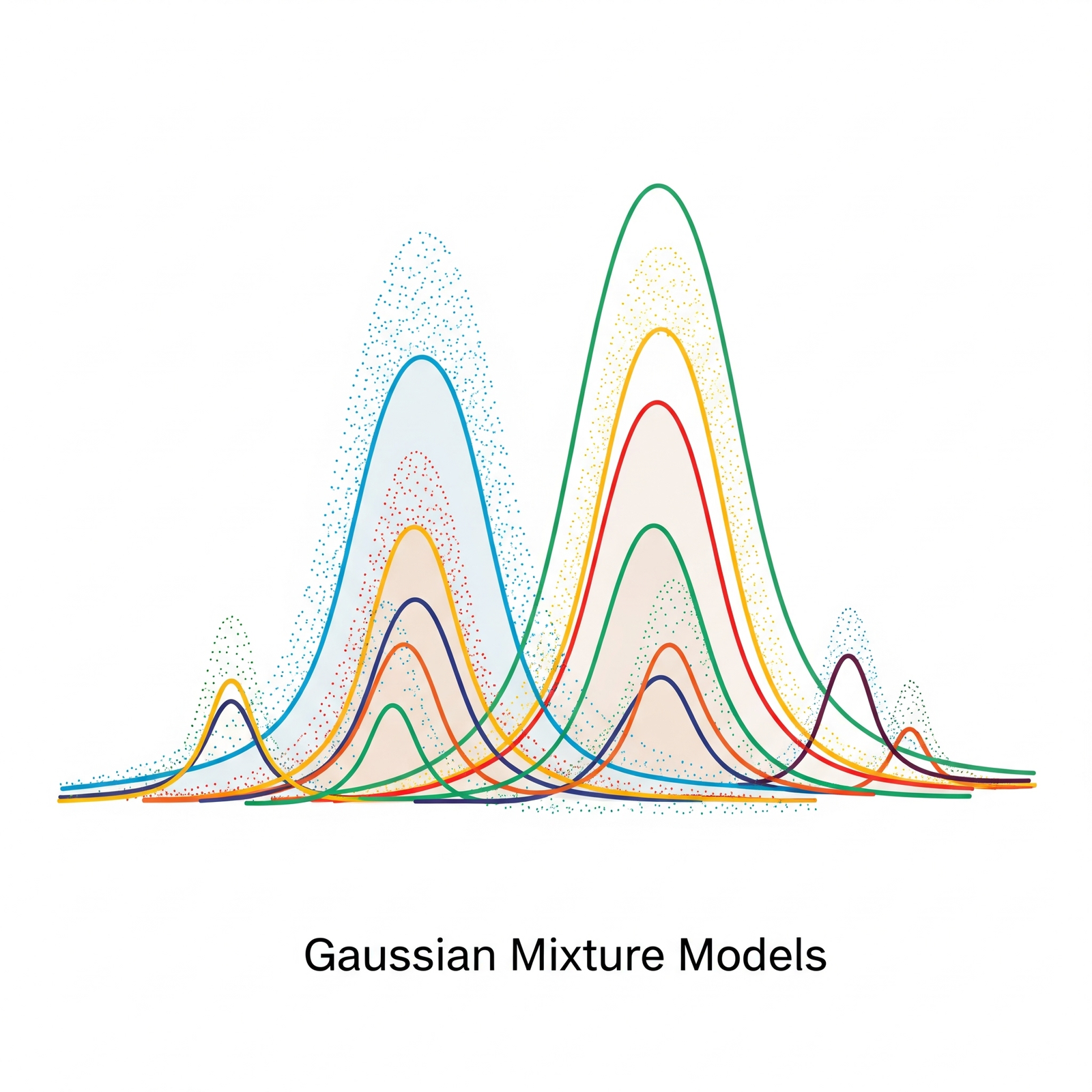
At its heart, a Gaussian Mixture Model assumes that your data points are generated from a mixture of several simpler probability distributions, specifically Gaussian (normal) distributions. Think of it like this: instead of assuming all adult heights come from one big bell curve, a GMM acknowledges that they might come from a “mix” of two smaller, distinct bell curves (one for each gender), summed together.

Each component Gaussian in the mixture has its own set of parameters:

• Mean (μ): The center of the Gaussian (e.g., the average height for a gender).
• Covariance Matrix (Σ): Describes the shape and orientation of the Gaussian (e.g., how spread out the heights are, and if they correlate with other features).
• Mixing Coefficient (π): Represents the weight or proportion of that particular Gaussian in the overall mixture (e.g., the percentage of males versus females in the population).

The beauty of GMMs lies in their ability to model complex, multi-modal data distributions by combining these simpler, well-understood Gaussian shapes.

Unlocking the Parameters: GMM Estimation via Expectation-Maximization (EM)

So, how do we find these optimal parameters (means, covariances, and mixing coefficients) for each Gaussian component that best explain our data? This is where the Expectation-Maximization (EM) algorithm comes into play.

Unlike simpler models where you can directly calculate parameters, with a GMM, we have a “chicken-and-egg” problem:

• If we knew which data point belonged to which Gaussian component, we could easily calculate the parameters for each Gaussian.
• If we knew the parameters of each Gaussian, we could easily figure out which data point most likely belongs to which Gaussian.

The EM algorithm tackles this iteratively:

1. Initialization: We start by making an educated guess for the parameters of each Gaussian (e.g., random means, identity covariances, equal mixing coefficients).
2. E-Step (Expectation): In this step, we calculate the “responsibilities.” For each data point, we determine the probability that it belongs to each of the current Gaussian components. This is a “soft” assignment – a data point might have a 0.8 probability of belonging to Gaussian 1 and a 0.2 probability of belonging to Gaussian 2.
3. M-Step (Maximization): Using these calculated responsibilities, we now update the parameters of each Gaussian component. We “maximize” the likelihood of the data given the responsibilities, essentially recalibrating each Gaussian’s mean, covariance, and mixing coefficient to better fit the data points it’s most “responsible” for.
4. Iteration: We repeat the E-step and M-step iteratively. With each iteration, the model’s parameters improve, and the “responsibilities” become more accurate, until the parameters converge (stop changing significantly).

EM is a powerful technique for models with hidden variables, and it’s the workhorse behind estimating GMM parameters.

GMM and K-means: A Tale of Two Clustering Algorithms

You might have heard of K-means, another popular clustering algorithm. Interestingly, there’s a strong connection between GMMs and K-means:

• Similarity: Both are iterative algorithms that aim to group data points into “clusters” based on their proximity to cluster centers (or components).
• K-means as a Special Case of GMM: K-means can be viewed as a simplified, “hard” version of a GMM. Specifically, K-means is equivalent to a GMM where:
  • The covariance matrices of all Gaussian components are spherical (i.e., data is spread equally in all directions) and identical.
  • The mixing coefficients of all components are equal.
  • Crucially, in K-means, each data point is hard-assigned to exactly one cluster (the closest centroid), rather than having a probabilistic “soft” assignment across multiple clusters as in GMM’s E-step.

Key Differences Summarized:

Feature	Gaussian Mixture Model (GMM)	K-means Clustering
Assignment	Soft (probabilistic) to multiple clusters	Hard (deterministic) to one cluster
Cluster Shape	Flexible (modeled by covariance matrix – can be elliptical)	Spherical (assumes clusters are circles/spheres)
Cluster Size	Can model clusters of different sizes	Tends to find clusters of similar variance/density
Overlapping	Handles overlapping clusters gracefully	Struggles with overlapping clusters
Computational Cost	Generally higher	Lower
Output	Probabilities of belonging to each cluster	Cluster assignment (label)

In essence, if K-means offers a quick sketch of your data’s groups, GMM provides a more nuanced, probabilistic, and geometrically flexible portrait of the underlying distributions, making it ideal for more complex data landscapes.