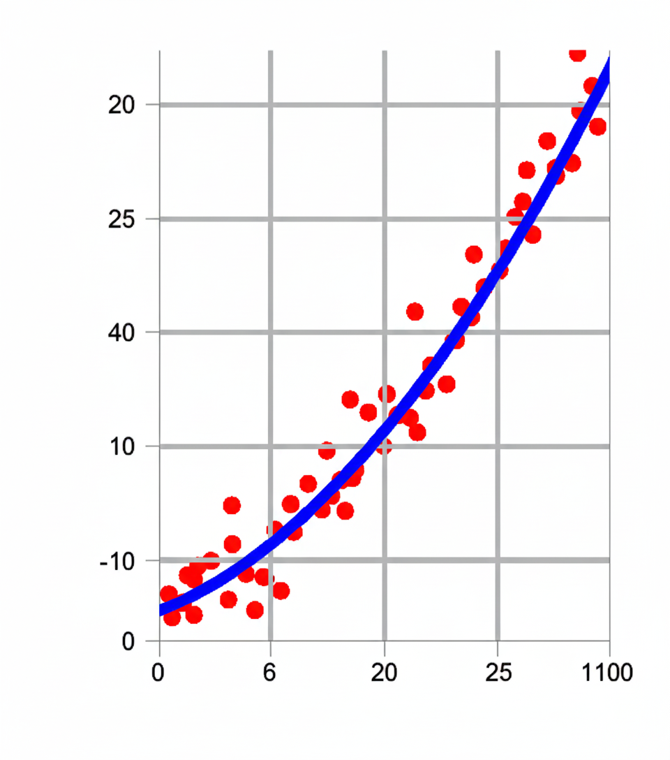
In linear regression, Ordinary Least Squares (OLS) is a powerful method for finding the best-fit line for a dataset. Its primary appeal is that it offers a closed-form solution, meaning you can calculate the ideal model parameters in a single step using matrix operations, rather than through an iterative process.
The OLS Approach
The core idea is to minimize the sum of the squared differences between the predicted values and the actual values. This process starts with setting up the problem in a linear regression model, where the output (like median house value) is a linear combination of input features (like median income).
This model is then represented in matrix form, with the target variables forming a vector y, the features forming a matrix X, and the parameters forming a vector θ. A crucial part of this setup is the inclusion of a column of ones in the X matrix. This allows the model to have an intercept term, giving the best-fit line the flexibility to move up or down, which is essential for accurate predictions in most real-world scenarios.
The objective is to find the parameter vector θ that minimizes the squared error. By taking the derivative of this error function with respect to the parameters and setting it to zero, we arrive at the closed-form solution.
The Drawback
However, the beauty of the closed-form solution comes with a major drawback. The solution requires a matrix inversion step. For small datasets, this is not a problem, but as the amount of data grows, this computation becomes extremely expensive and can be a significant practical bottleneck. This limitation is the primary reason why alternative methods, such as iterative approaches like Stochastic Gradient Descent, are needed for large-scale machine learning problems.
The Solution: Stochastic Gradient Descent (SGD)
Unlike OLS, Stochastic Gradient Descent (SGD) is an iterative method that finds the solution by taking many small, incremental steps. Instead of solving for parameters directly, it starts with an initial guess and continuously updates the parameters to minimize a loss function, typically the Mean Squared Error (MSE).
A toy example for practicing by hand to learn SGD with a smaller learning rate of 0.01 for better understanding:
Initial Setup:
Data table:
| Income(X) | Price(y) |
|---|---|
| 2 | 4 |
| 4 | 6 |
Points: (2,4) and (4,6)
Initial θ = [1, 1]
MSE = 1.0
Iteration 1 (learning rate = 0.01):
Gradient = -[1, 3]
New θ = [1,1] – 0.01×[-1,-3] = [1.01, 1.03]
Predictions: 3.07, 5.13
Errors: -0.93, -0.87
MSE = (0.8649 + 0.7569)/2 ≈ 0.811
Iteration 2:
θ = [1.01, 1.03]
Gradient = -[-0.8, -1.54]/2 = [0.4, 0.77]
New θ = [1.01,1.03] – 0.01×[0.4,0.77] = [1.006, 1.0223]
Predictions: 3.0506, 5.0952
Errors: -0.9494, -0.9048
MSE ≈ 0.857
Iteration 3:
θ = [1.006, 1.0223]
Gradient = -[-0.8542, -1.6186]/2 = [0.4271, 0.8093]
New θ = [1.006,1.0223] – 0.01×[0.4271,0.8093] = [1.0017, 1.0142]
Predictions: 3.0301, 5.0595
Errors: -0.9699, -0.9405
MSE ≈ 0.913
Observation: The MSE is increasing, which suggests the learning rate might still be too large. Let’s try an even smaller learning rate of 0.001. With learning rate = 0.001:
Iteration 1:
New θ = [1,1] – 0.001×[-1,-3] = [1.001, 1.003]
Predictions: 3.007, 5.013
Errors: -0.993, -0.987
MSE ≈ 0.981
Iteration 2:
Gradient = -[-0.98, -1.94]/2 = [0.49, 0.97]
New θ = [1.001,1.003] – 0.001×[0.49,0.97] = [1.00051, 1.00203]
Predictions: 3.00457, 5.00863
Errors: -0.99543, -0.99137
MSE ≈ 0.983
Iteration 3:
Gradient = -[-0.9868, -1.9606]/2 = [0.4934, 0.9803]
New θ = [1.00051,1.00203] – 0.001×[0.4934,0.9803] = [1.0000166, 1.0010497]
Predictions: 3.002116, 5.0042158
Errors: -0.997884, -0.9957842
MSE ≈ 0.995
Key Takeaways:
- The learning rate significantly impacts convergence
- A smaller learning rate (0.001) provides more stable updates
- The error decreases gradually with a smaller learning rate
- More iterations would be needed to reach the optimal solution
Refining the Process: Advanced Techniques
To make the training process even more efficient, advanced techniques are often used. Early stopping halts the training when the model’s performance on a separate validation set stops improving, which prevents overfitting and saves computational time. Additionally, learning rate back-off automatically reduces the learning rate when the model’s performance plateaus, allowing it to take smaller, more precise steps as it fine-tunes the parameters near the minimum.
In conclusion, while OLS offers a fast, guaranteed solution for small datasets, it can’t handle the scale of modern machine learning problems. SGD is a more versatile, memory-efficient, and computationally cheaper approach that makes linear regression feasible for massive datasets.
