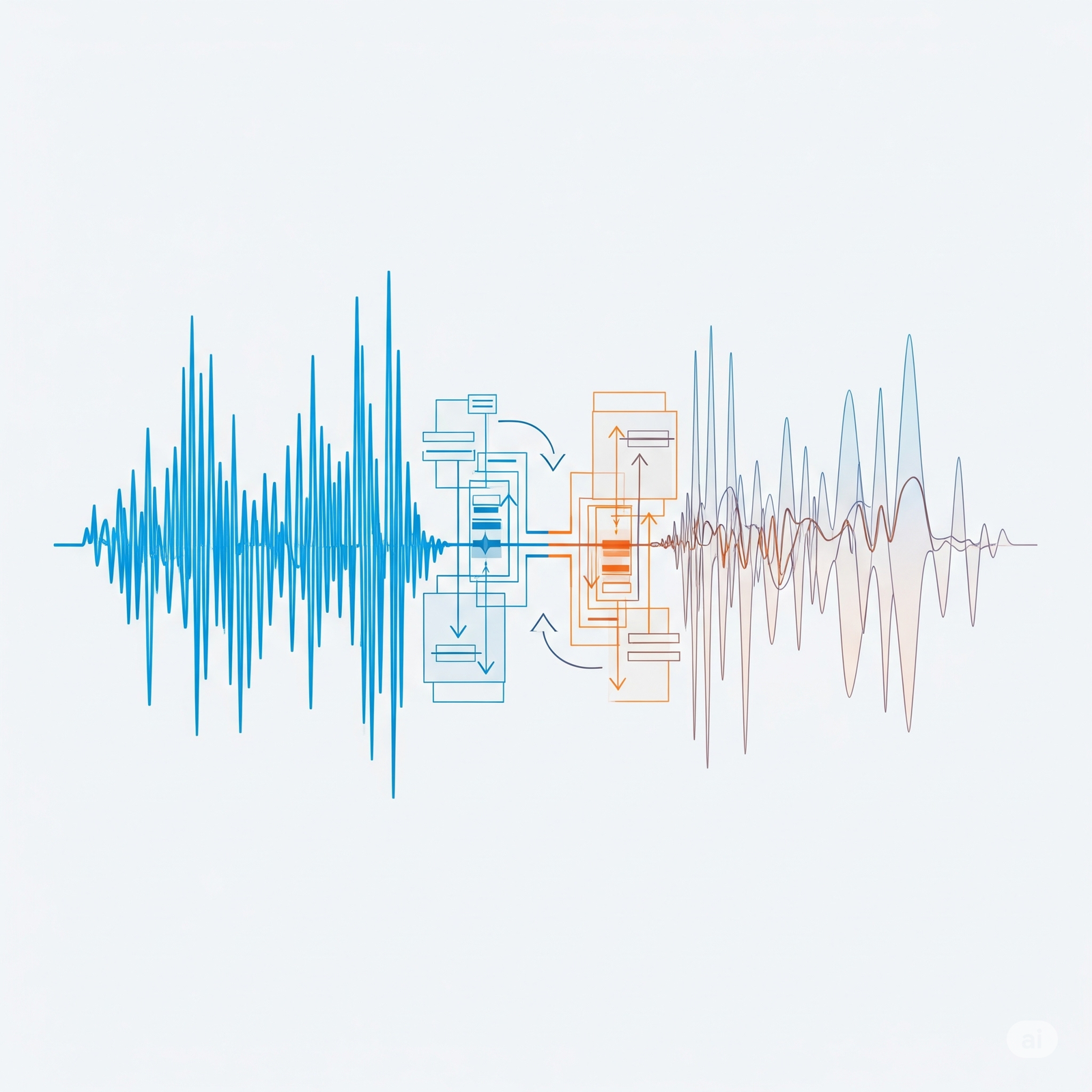
Signal processing is a fascinating field that allows us to synthesize, transform, and analyze signals, with a particular focus on sound. In our modern digital world, converting continuous analog sound into discrete digital data is a crucial first step for many applications, from streaming music to speech recognition systems. This process is known as sampling, and its inverse is reconstruction.
Let’s break down these fundamental concepts.
Step 1: The Sampling Process
Sampling is the procedure of measuring an analog signal at a series of points in time, typically with equal spacing. When you record audio, for instance, an analog-to-digital converter (ADC) takes these measurements from the microphone’s output.
- Conversion to Digital Form: The primary objective of speech coding, or simply coding, is to efficiently represent speech signals digitally. This allows for bandwidth efficiency when transmitting the signal over communication channels or storing it on various media like tapes and disks.
- Mathematical Representation: Consider a continuous-time analog signal, denoted as \(x_a(t)\). When this signal is sampled, we obtain a discrete-time signal \(x(n)\) (or \((x[n]\)). The sampling process can be mathematically represented as multiplying the analog signal by a train of Dirac delta impulses. If the sampling instances are defined by \(t_n = nT + t_0\), where \(T\) is the sampling period and \(t_0\) is an initial time shift, the sampled signal \(y(t)\) can be written as: \(y(t) = \sum_{n=-\infty}^{+\infty} x_a(t_n)\delta(t-t_n)\) The discrete samples are then \(x[n] = x_a(nT + t_0)\).
- Sampling Rate (\(f_S\)): This is the number of samples taken per second, and it is the reciprocal of the sampling period (\(f_S = 1/T\)). Common sampling rates for audio include 44.1 kHz for “CD quality” sound and 48 kHz for DVD sound. Applications beyond audio might require higher rates to capture higher frequencies.
- Effect in the Frequency Domain: When a signal is sampled in the time domain, its Fourier Transform undergoes a significant transformation. If \(X_a(j\omega)\) is the Fourier Transform of the continuous signal \(x_a(t)\), the Fourier Transform of the sampled signal, \(Y(j\omega)\), becomes a periodic replication of \(X_a(j\omega)\). For \(t_0=0\), this relationship is given by: \(Y(j\omega) = \frac{1}{T} \sum_{k=-\infty}^{+\infty} X_a(j(\omega – k\Omega))\) where \(\Omega = 2\pi/T\) is the angular sampling frequency. This equation shows that the original spectrum \(X_a(j\omega)\) is repeated at integer multiples of the sampling frequency \(\Omega\).
Understanding Aliasing: The Pitfall of Undersampling
A critical concept to grasp during sampling is aliasing.
- What is Aliasing?: When the spectral copies created during sampling overlap, information about the original spectrum is lost, and we refer to this as aliasing. For example, if a signal is sampled at 10,000 Hz, a 5500 Hz component becomes indistinguishable from a 4500 Hz component.
- Folding Frequency (Nyquist Frequency): The point at which frequencies above it get aliased is called the folding frequency, which is half of the sampling rate (\(f_S/2\) or \(\pi/T\)).
- The Nyquist-Shannon Sampling Theorem: To prevent aliasing and ensure perfect reconstruction, a fundamental principle known as the Nyquist-Shannon Sampling Theorem must be observed. This theorem states that if a signal contains no energy at frequencies above half of the sampling rate (\(f_c < f_S/2\) or \(\omega_c < \pi/T\)), the original signal can be recovered exactly. This means that the sampling frequency \(f_S\) must be at least twice the maximum frequency component (\(f_c\)) present in the analog signal, i.e., \(\mathbf{f_S \ge 2f_c}\). If this condition is violated, the replicated spectra will overlap, and the higher frequencies will “fold back” into the lower frequency range, creating an irreversible distortion.
- Anti-Aliasing Filter: To prevent aliasing, it is good practice to filter out frequencies above the folding frequency before sampling. A low-pass filter used for this purpose is known as an anti-aliasing filter.
Step 2: The Reconstruction Process (Interpolation)
Once a signal has been digitized, the ultimate goal for the user is often to convert it back to its analog form. This process is known as reconstruction or interpolation.
- Removing Spectral Copies: Reconstruction involves applying a low-pass filter – often referred to as a “brick wall filter” due to its ideal frequency response – to remove the spectral copies that were introduced by sampling. An ideal low-pass filter \(H(j\omega)\) would have a transfer function defined as: $$H(j\omega) = T \cdot \text{rect}\left(\frac{\omega}{2\omega_c}\right) = \begin{cases} 1 & \text{for } |\omega| \le \omega_c \ \\ 0 & \text{for } |\omega| > \omega_c \end{cases}$$ where \(\omega_c = \pi/T\) is the cutoff frequency, exactly at the folding frequency.
- Perfect Reconstruction with Sinc Function Interpolation: If the original signal was “bandwidth limited” (meaning it contained no energy above half the sampling rate) and sampled correctly (adhering to the Nyquist criterion), it’s possible to recover the original signal exactly. This can be achieved by summing shifted and scaled copies of the sinc function, which effectively interpolates between the sampled values. The continuous signal \(x_a(t)\) can be reconstructed from its discrete samples $$x[n] as: x_a(t) = \sum_{n=-\infty}^{+\infty} x[n] \cdot \text{sinc}\left(\frac{t-nT}{T}\right)$$ where \(\text{sinc}(x) = \frac{\sin(\pi x)}{\pi x}\). This principle relies on properties of the sinc function related to the orthogonality of sinc functions at integer multiples, as highlighted in the sources.
In summary, proper sampling ensures that the analog information is faithfully captured in digital form by adhering to the Nyquist criterion and preventing aliasing. Careful reconstruction then allows for the precise recreation of the original signal by filtering out redundant spectral copies and interpolating the discrete samples back into a continuous waveform.